
Exponentials vs. Power Laws

How can you predict how a person learns over a given amount of time? How does an ML model learn? Why do loss curves look like that, and what does that have to do with human learning? These are questions I am aiming to answer here. I should warn you ahead of time that if you aren't comfortable with CS related math, this will probably be a slightly more difficult read than other things I have written.
Brief Note About Math Rendering
The math rendering in Substack is a bit limited. Inlining LaTeX doesn’t appear to be an option right now, so I will have to make do by avoiding inlined equations, and bolding and italicizing some of the inlined variables that I use for the sake of readability.
General Curves
Curves that look like the following exist in many real world contexts:
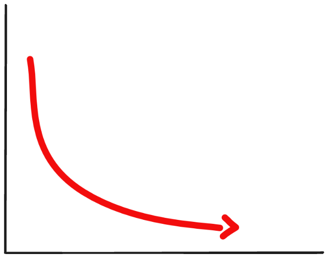
However, there are multiple ways of modeling this. The two that I will focus on are the exponential decay function,
given some constant, α, and the power law,
given some constants, α and β and some offset, μ.
The reason it is relevant to machine learning is apparent if you've seen a loss curve mapped out. This is what it looks like for reference:
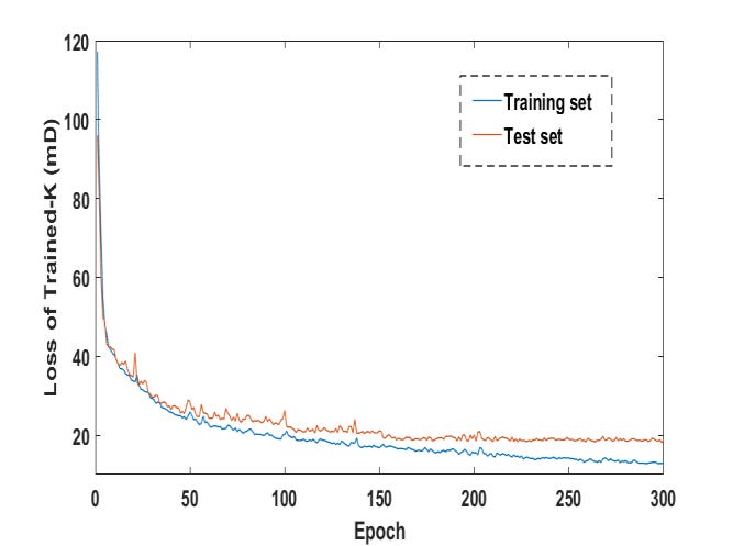
These look similar, and you could be forgiven for thinking that this similarity is only superficial. The real curve is messy after all, and real life tends to be chaotic. That being said, there is a real connection between these types of functions.
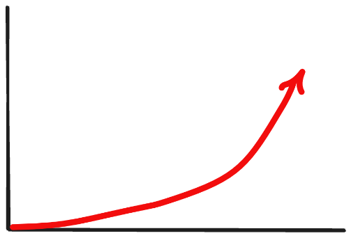
It is worth mentioning explicitly that I am assuming that α and β are not necessarily positive, so in cases of exponentials where α < 0, and power law functions where β < -1, we can also get curves that look like this:
Exponential Decay
Let's say you are studying for a test, and there is a list of words that you need to learn. You make flash cards, and start iteratively going through the deck, guessing and checking each word. Each time you go through the deck, after iteration, t, there is a probability, p, of learning each word. Given this setup, you would expect the proportion of words you don't know at iteration t to be:
This is because the probability of a word that hasn't been learned yet, not being one of the words that gets learned each round is:
This means that the function that predicts the number of words you learn will behave like an exponential decay function. If you stopped here, you'd think that that is how learning works. It even makes sense because exponential decay functions asymptotically approach zero, just like loss functions.
In practice, functions that accurately predict skill acquisition seem to be best predicted by power laws. The Stanford-B power law function appears to be particularly good at predicting skill acquisition. Why might this be? In an abstract sense, it seems like exponential decay should be the best predictor. If something seems like it should be exponential, and it is actually predicted by t to some exponent.
Graph Traversal
Imagine that we have a graph with evenly spaced nodes laid out over a 2D space, and we are doing a BFS-style search, except every iteration, we explore all nodes that are connected to the explored part of our graph (rather than one at a time).
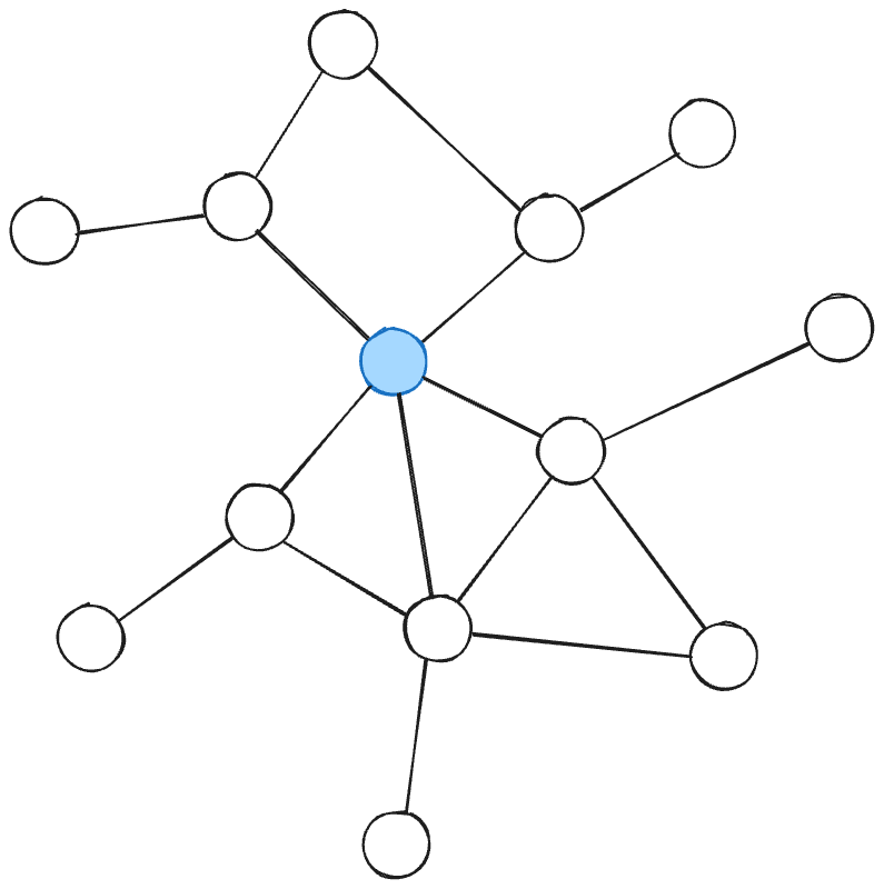
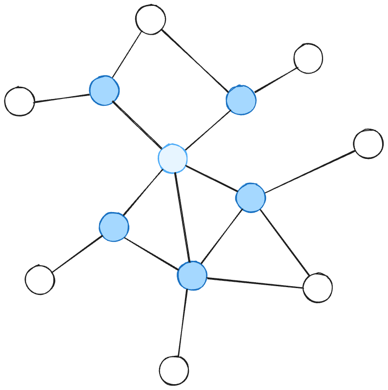
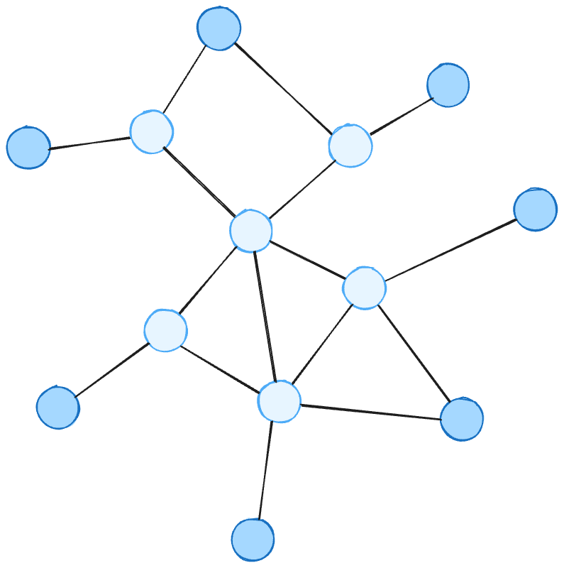
If you try to guess how many nodes it will uncover naively, you would might repurpose the formula,
which is what is usually used to predict the number of game positions considered given some branching factor, b, and desired depth, d.
In the case of a game where each player has three possible decisions each turn, a search over all possible states of the game tree, after two players have taken turns moving, would look like this:
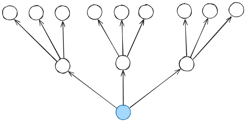
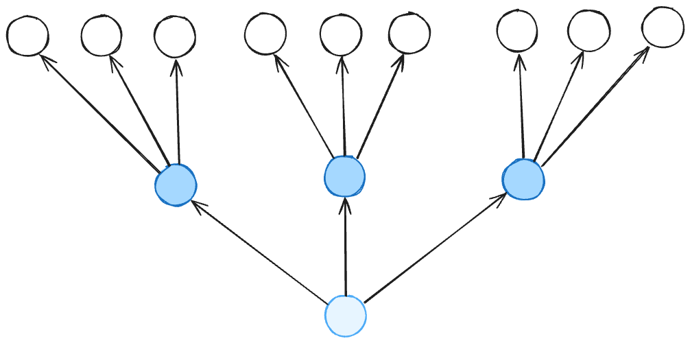
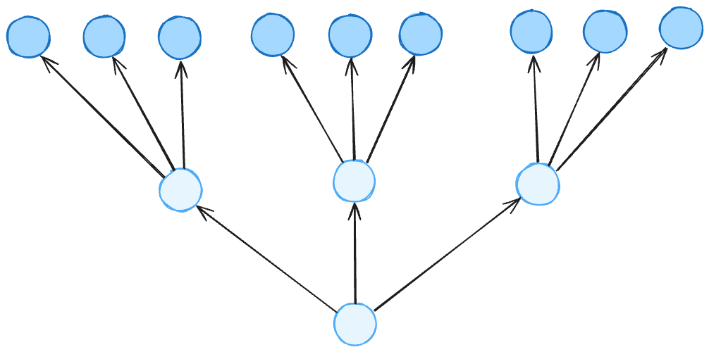
This would give us an exponential like we saw before:
if b is the average number of connections each node in the 2D graph has. Maybe you could consider any overlapping frontier nodes to be negligible.
However, we can look at it a different way. Let's consider an example of a similar graph search, but this time, the nodes of the graph are arranged into a grid. We pick a point at the center of the grid, and explore the graph starting from there. You would think based on our above logic, because each node has 3 to 4 neighbors (4 minus one that has already been explored on the way there), the number of nodes covered would be somewhere between
and
Let's look at what this actually looks like:
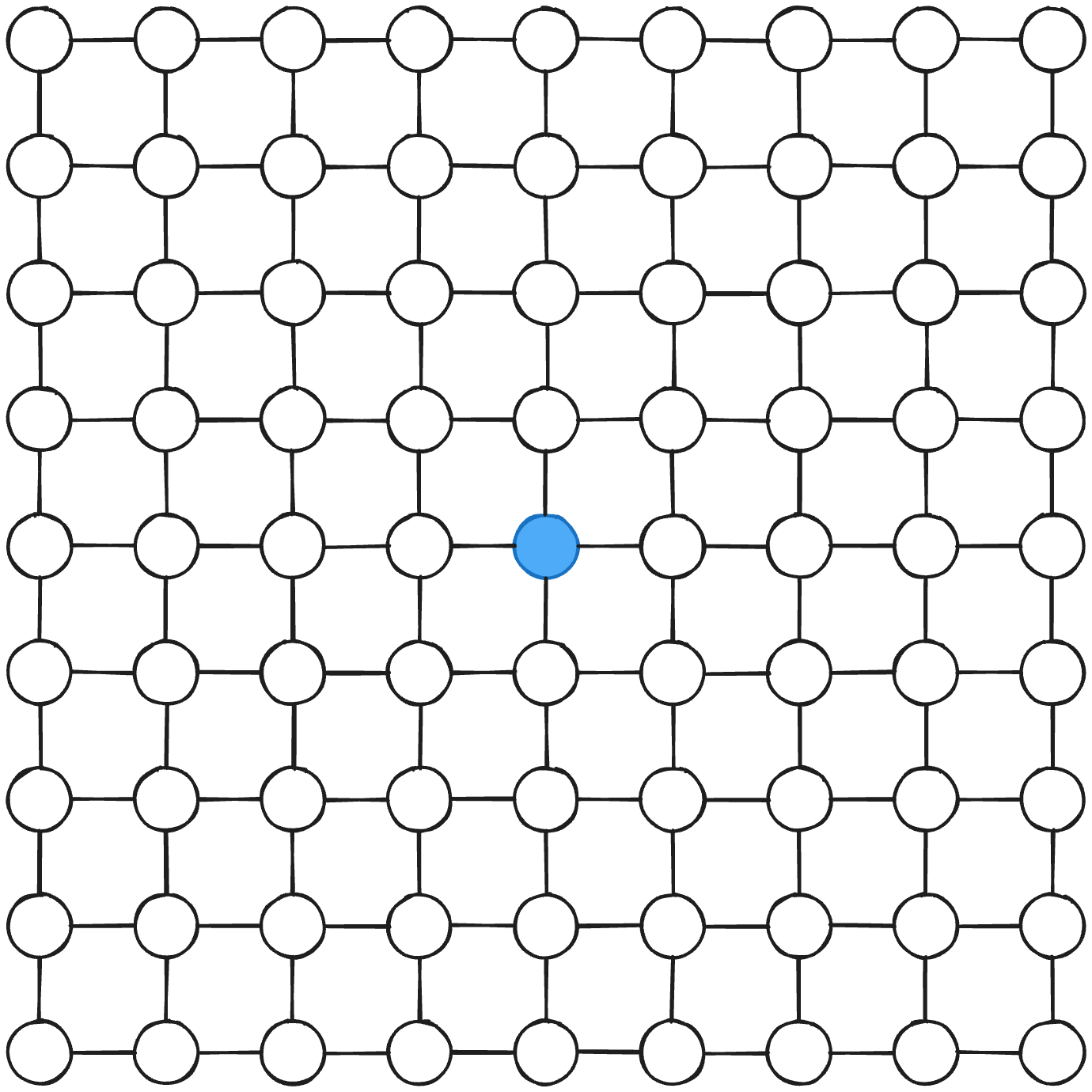
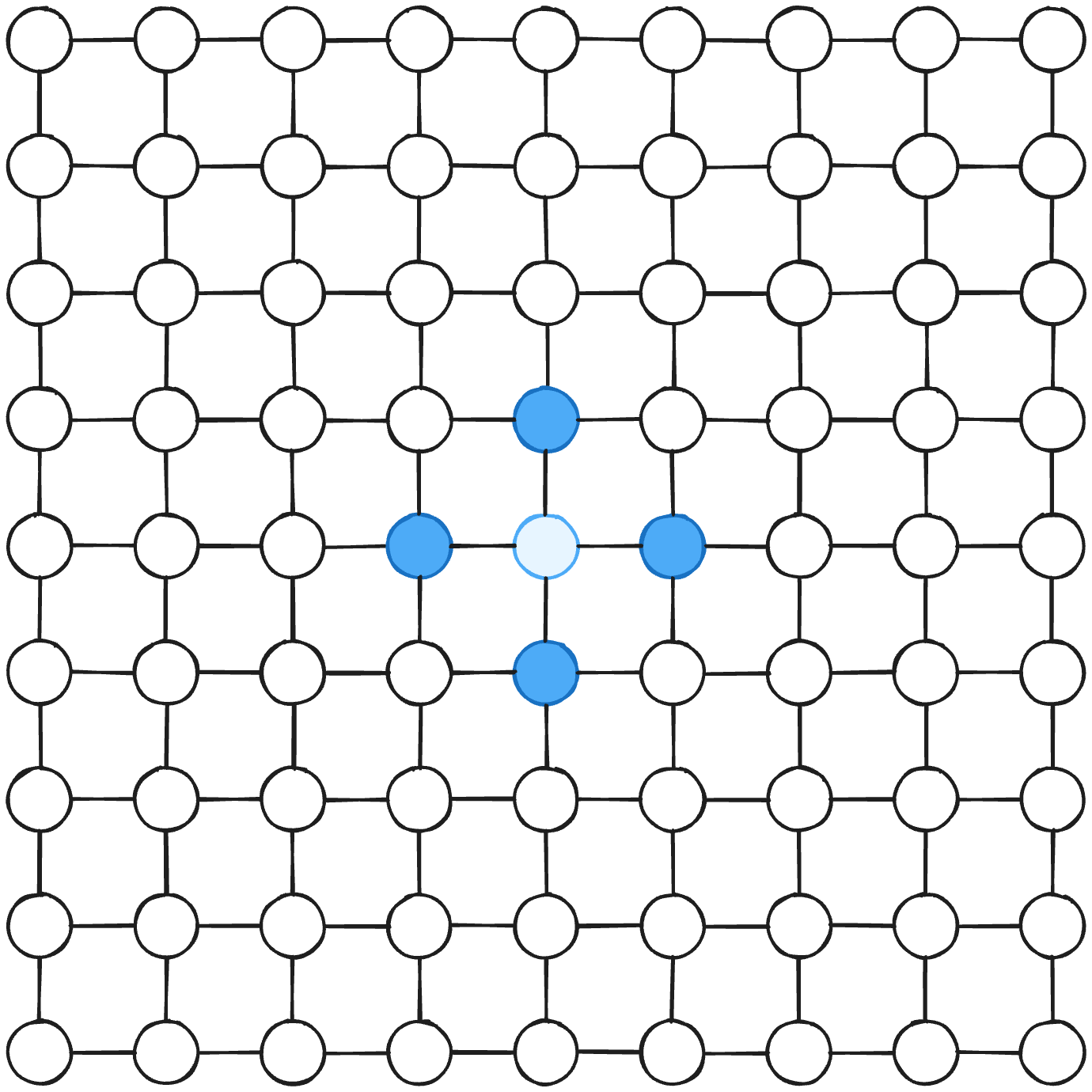
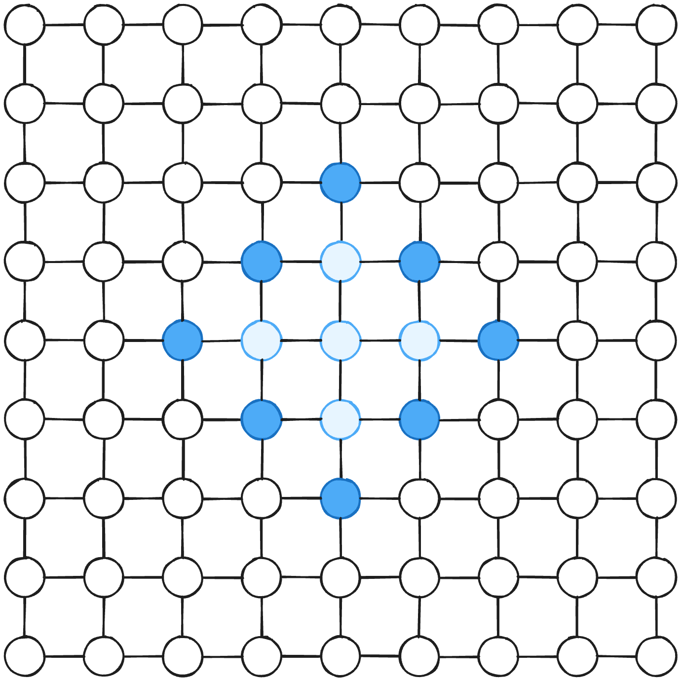
In this case, it becomes apparent that the number of nodes explored at t is proportional to the area of an expanding square.
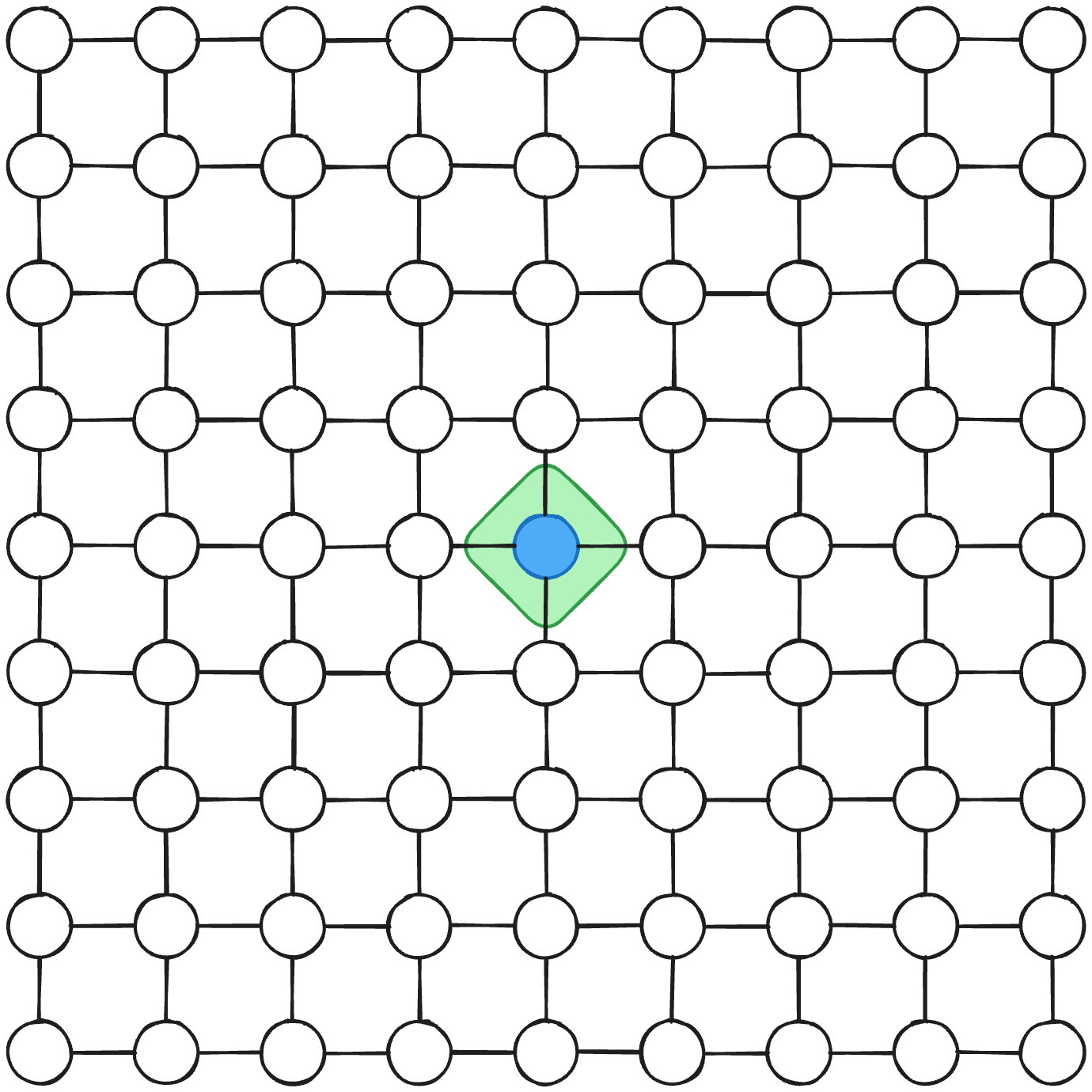
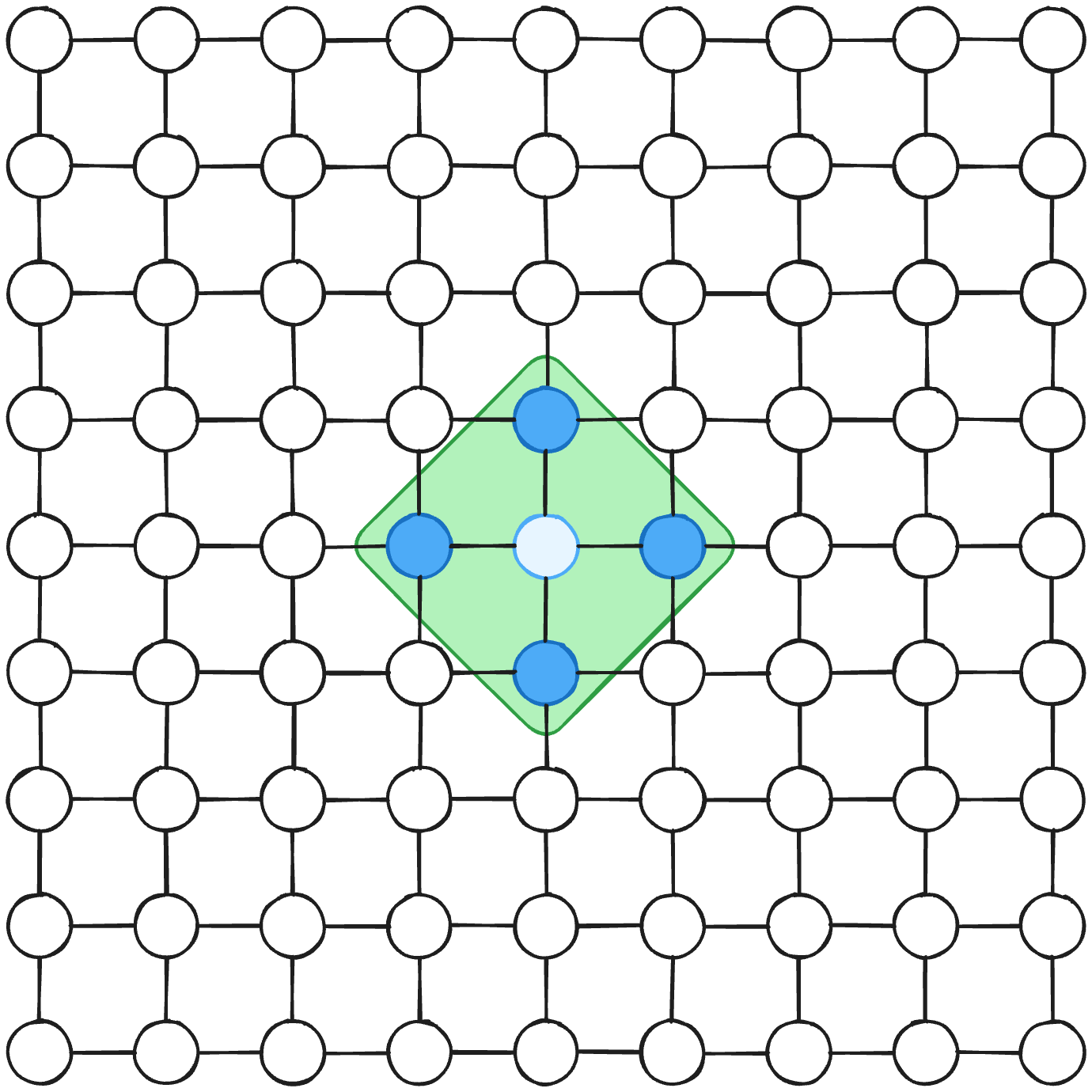
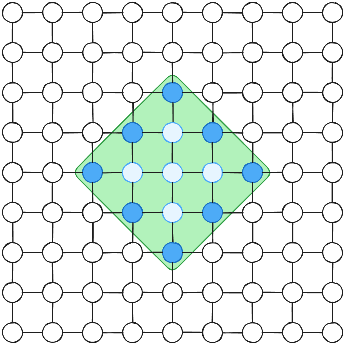
This means that the function would be
or a quadratic function of t.
The reason for this seeming mismatch is that there are overlapping frontier nodes at each moment. Below is an example with overlapping nodes in green:
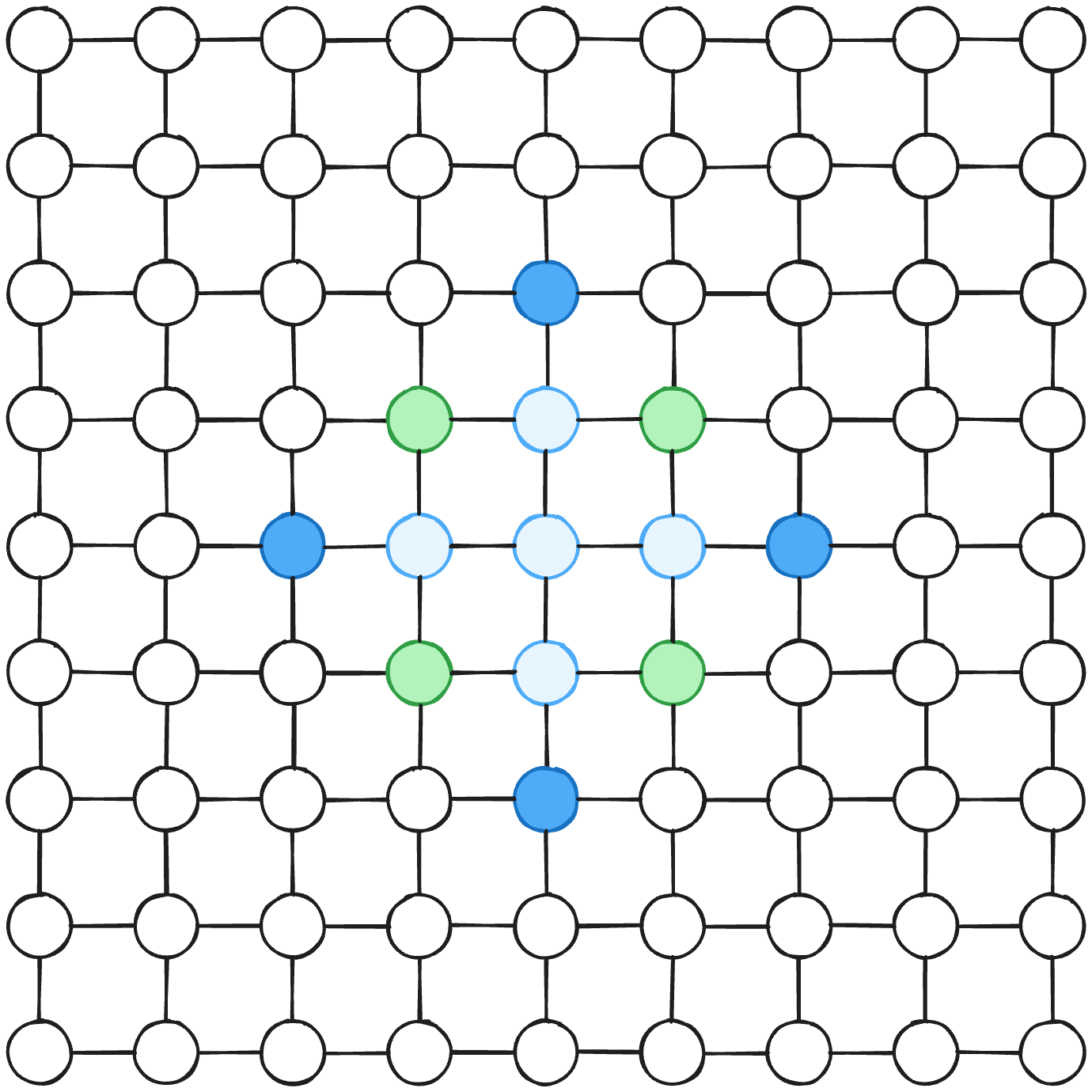
This means that as the explored part of the graph increases, some of the branches go to the same places or places that have been explored already, which means that there are redundancies in what is added at each step in the naive version. We can describe these redundancies as a function of t, or r(t), with the equation,
which becomes
If you reframe this as something like a time complexity problem, it becomes apparent that r(t) would have to behave like an exponential, meaning that the number of redundancies will exponentially increase with t. Exponential growth is happening, but it is canceled out by redundancies that are also exponentially increasing, which results in polynomial growth.
This illustrates how something that looks like it should be exponential is actually polynomial, the reason being because there are overlaps between the connected nodes at each step. Ultimately, this will happen any time the expansion of something is constrained in such a way that exponential increases are canceled out. This happens in learning when the thing being learned behaves more like a landscape that we are traversing or an area that we are covering, and less like unbounded exponential growth.
The Real World
Practically, this might look like us finding two distinct paths to the same conclusion or fact about something. A few examples:
If we find some bones during an archeological dig, we can figure out the age with carbon dating, or by checking the layer of dirt the bones were buried under.
We can estimate the size of the earth with Eratosthenes’ Method, or by measuring the dip in the horizon on top of a mountain when compared to sea level, among other methods.
There are multiple ways to prove the Pythagorean theorem.
These are all analogous to redundant frontier nodes in our example above. This is likely why learning and discovery in real-world cases is often best described by a power law.
You might be wondering what this all means. The answer would be that real world learning looks very similar to landscape traversal, and is you see something like that in a context where you are looking for facts that you can derive from other facts, you should be able to find the analogue of redundant frontier nodes somewhere. It also means that if learning, knowledge acquisition, or loss function of something looks more like an exponential decay function, bits of information that are learned are likely more unconnected from each other, and the learning of each of them is probably happening independent of the others.
This isn't just an abstract way of thinking about learning either. It would imply that error as a function of time during skill acquisition will usually look more like a function described by a power law, and so will learning in areas of study where facts are deeply entangled with each other. On the other hand, error functions associated with the learning of disconnected facts by rote will tend to look more like exponential decay functions. This might be why rote learning is faster, even though it is less generally applicable.